The use of spectral data to predict soil organic matter in European soils

Soil organic matter

Soil organic matter (SOM) is the fraction of the soil that consists of plant and animal detritus (remains, waste products and other organic debris) at various stages of decomposition (breakdown), cells and tissues of soil microbes, and substances that soil microbes synthesize. It is estimated that concentration of SOM in most of the productive agricultural soils ranges between 3 % and 6 %. Even though it is only a small part of soil organic matter contributes to soil productivity in numerous ways and the various components of organic matter influence different properties of soil.

From the chemical point of view SOM is composed mainly of just a few chemical elements namely carbon, hydrogen and oxygen. These elements together make almost 92 % of all SOM. However, organic matter also contains small amounts of other essential elements, such as nitrogen, phosphorus, sulfur, potassium, calcium and magnesium which are encompassed in organic residues.\A0

Generally, SOM is divided into living and dead components which can range from very recent inputs, such as stubble, to largely decayed materials that are thousands of years old. It is estimated that about 10 % of below-ground SOM, such as roots, fauna and microorganisms, fall into the living category (see Fig. 1).

It is normally considered that SOM is made up of different components which vary widely in size, turnover time and composition in the soil. These components can be grouped into four major types:

1. Dissolved organic matter;

2. Particulate organic matter;

3. Humus;

4. Resistant organic matter.

Fig. 1. Composition of soil organic matter.

The living organic matter includes such parts as the microorganisms responsible for decomposition (breakdown) of both plant residues and active soil organic matter or detritus. Organic compounds in vegetal detritus includes carbohydrates which range in complexity from simple sugars to the complex molecules of cellulose, fats that are composed of glycerides of fatty acids, like butyric, stearic, and oleic, lignins that are complex compounds, formed from the older parts of wood, and are resistant to decomposition, proteins, and charcoal. Humus is the stable fraction of the soil organic matter that is formed from decomposed plant and animal tissue and is the final product of the decomposition processes. The first two types of organic matter (dissolved organic matter, particulate organic matter) contribute to soil fertility because the breakdown of these fractions results in the release of plant nutrients such as nitrogen, phosphorus, potassium, etc. The humus fraction has less influence on soil fertility because it is the final product of decomposition. Therefore, humus is also called the stable organic matter. However, it still has much importance to soil fertility because it contributes to soil structure, soil tilth, and cation exchange capacity. This is also the fraction that darkens the soil\92s color.

There are many benefits of soil organic matter in an agricultural soil. These benefits can be grouped into three categories:

Physical Benefits

● Enhances aggregate stability, improving water infiltration and soil aeration, reducing runoff.

● Improves water holding capacity.

● Reduces the stickiness of clay soils making them easier to till.

● Reduces surface crusting, facilitating seedbed preparation.

Chemical Benefits

● Increases the soil\92s cation-exchange capacity or its ability to hold onto and supply over time essential nutrients such as calcium, magnesium and potassium.

● Improves the ability of a soil to resist pH change (also known as buffering capacity).

● Accelerates decomposition of soil minerals over time, making the nutrients in the minerals available for plant uptake.

Biological Benefits

● Provides food for the living organisms in the soil.

● Enhances soil microbial biodiversity and activity which can help in the suppression of diseases and pests.

● Enhances pore space through the actions of soil microorganisms. This helps by increasing infiltration and reducing runoff.

Evaluation of soil organic matter concentration

Due to the forementioned benefits of soil organic matter it is regarded as one of the key parameters (characteristics) of soil and is measured routinely to monitor the soils health and condition. Due to the complexity of the composition of soil organic matter it is difficult to directly evaluate its amount. This is why most often the concentration of SOM in soil is determined first by determining the total carbon content - soil organic carbon (SOC). Then SOM is evaluated from the calculated value of SOC. The calculation between the concentrations of SOC to SOM has historically formed to be a simple act of multiplication by a constant \A0(van Bemmelen factor):

The value of the constant \A0is derived from the assumption that soil organic matter is comprised of 58 % of carbon. However, throughout the years the legitimacy of this value was put under question. Several studies have shown that the conventional carbon-to-organic matter conversion factor is too low for universal application and fails to account for the significant variation in the carbon content of soil organic matter. Therefore, there have been many suggestions on what value of the constant should be used for soils regarding their composition (see Table 1).

Table 1. The evaluated values of conversion factor in different countries and soils (D. W. Pribly, 2010).

Country	Soil description	Factor value			Reference
		Low	Average	High
Belgium	Soils (rich in organic matter)	1.44	2.05	3.10	De Leenheer et al. (1957)
Denmark	Forest	1.55	2.63	15.4	Christensen and Malmros (1982)
England	Mineral; agricultural	2.52	3.45	14.1	Warrington and Peake (1880)
England	Forest; Wetlands	1.78	2.07	3.62	Howard (1964)
Europe	Forest; grass; peat	1.97	2	2.5	Ponomareva and Plotnikova (1967)
US	Mineral	1.63	1.92	2.14	Alexander and Byers (1932)
Wales	Peat	1.86	1.88	1.95	Robinson et at. (1929)
Wales	Mineral and organic	1.74	2.73	5.64	Ball (1964)
Worldwide	Mineral and organic	1.35	1.74	2.44	Robinson (1927)
Worldwide	Surface soils	1.9	2.2	2.5	Broadbent (1953)

Various experimental and theoretical studies were performed in order to evaluate the optimal value of the conversion factor and one of the most suggested value is \A0(Douglas W. Pribly, 2010).

The standard practice for determining organic carbon is performing chemical analysis of the soil. This method involves a lot of procedural tasks and chemical reagents but provides an accurate value of the SOC. However, the time and economic resources needed for such analysis are not favorable because the evaluation of SOM cannot be efficiently upscaled for larger fields or continuous monitoring. Such drawbacks of the standard SOC analysis techniques led to the emergence of other SOM evaluation techniques. One of them \96 hyperspectral or multispectral spectroscopy, has gained a lot of traction in the past decade and is becoming more and more applied for determination of all sorts of soil parameters (citation).

Hyperspectral and multispectral imaging

Hyperspectral imaging (HSI) spectroscopy is a modern and informative method belonging to the larger group of spectroscopy and spectral photography methods. Hyperspectral imaging technology is based on detection of the electromagnetic radiation reflected (most often) from the analyzed object (sunlight is usually used as the source of radiation) and collected in a vast range of spectral bands. The reflected light is detected using passive type scanning or snapshot sensors. Hyperspectral imaging spectroscopy is a remote sensing method which differs from other non-destructive remote spectroscopy methods in that during the scanning or instantaneous capture procedures a three-dimensional data array (so called hyperspectral cube) is generated. Hyperspectral cube can essentially be described as a three-dimensional data format where two dimensions (let\92s say x-axis and y-axis) describe the spatial coordinates and the third dimension (z-axis) describe the spectral coordinates (wavelength). One hyperspectral image can have tens or hundreds of spectral bands and each pixel of the image presents the reflected and sensor-recorded electromagnetic radiation intensity. Depending on the design and technical parameters, hyperspectral sensors can record information starting with ultraviolet light part of the spectrum (wavelength from around 200 nm) and ending in the long-wave infrared light (wavelength up to 15 μm). Hyperspectral imaging technology due to its informativeness and ease of application is used in many different fields: medicine, food industry, material property research, natural resource exploration, land on the farm, etc. Such a wide range of applications is provided by the physical nature of the method, which can be briefly described as the fundamental interaction of the electromagnetic radiation and matter (in terms of molecular structures). Because of this, hyperspectral imaging spectroscopy can be applied to study the spectral properties of light reflected by objects under study in order to identify the molecular compounds, determine their chemical and physical properties.

Close to hyperspectral, but simpler, and at the same time more primitive and less informative, technology is multispectral photography. In the latter, spectral images are generated by collecting the radiation data in much wider (several tens of nanometers and more) spectral bands. In contrast to hyperspectral sensors, multispectral sensors do not cover the full spectral range of the camera operation range. A fairly simple comparison of the hyperspectral and multispectral imaging results is presented in Fig. 2.

Fig. 2. Comparison of the data collected using multispectral (left) and hyperspectral (right) imaging methods.

In regard to the quality of the hyperspectral images, three main resolution parameters which determine the level of gathered information can be described. These are:

● Spatial resolution;

● Spectral resolution;

● Temporal resolution.

Spatial resolution is described as the smallest discernible detail in an image. It can be regarded as the dimension of the smallest object in an image that can be distinguished as an individual part. Spatial resolution is directly related to the clarity of the image. However, it should be mentioned that spatial resolution should not be mixed up with the number of pixels in an image. The spatial characteristics of a hyperspectral image depend on the design of the imaging sensor in terms of its field of view and the altitude at which the image is captured. If we consider that a finite patch of the ground is captured by each detector in a remote imaging sensor then the spatial resolution is inversely proportional to the patch size. Therefore, the smaller the size of the patch, the higher details can be interpreted from the observed scene.

Spectral resolution is defined as the number of spectral bands in the whole range of electromagnetic spectrum captured by the sensor. For example, the sensor might collect the light in a large frequency range but still have a low spectral resolution if the information is gathered from a small number of spectral bands. On the contrary, if a sensor collects the data from a small frequency range but captures a large number of spectral bands, high spectral resolution is obtained. In such cases it is possible to distinguish between two similar elements (having similar spectral features). Multispectral images, therefore, have a low spectral resolution and using this method it is not possible to resolve finer spectral signatures present in the analyzed area. HSI sensors acquire images in numerous continuous and extremely narrow spectral bands in mid infrared, near infrared and visible parts of the electromagnetic spectrum. This type of advanced imaging system shows tremendous potential for material identification on the basis of their unique spectral signatures. Spectrum of a single pixel in a hyperspectral image can give considerably more information about the surface of the material than a normal image. It is worth mentioning that even though multispectral imaging does not have as high spectral resolution as hyperspectral imaging, oftentimes it is much more practical to use. For example, in some cases it can be known for certain in which specific parts of the electromagnetic spectrum largest variations or differences between the spectral information of the analyzed objects are present. Therefore, collecting the information in the whole spectral range does not provide any more useful information and only burdens the analysis by adding redundant information.

Temporal resolution is considered if routine measurements of hyperspectral or multispectral remote sensing are made. In such cases depending on the type of information acquisition method the temporal resolution can depend on the orbital characteristics of the imaging sensor or the period of the experimental tests. Generally, the temporal resolution can be defined as the time needed to revisit and obtain data from the exact same location. Therefore, temporal resolution is considered high if the period between two measurements of the exact same location is short and is considered low if the said period is long. In general practice this parameter is defined in days.

Collection of the spectral data

Remote sensing applications provide unprecedented data streams for the retrieval and hence allow the monitoring of SOC across the VNIR\96SWIR spectral range. The different sensors used to collect the spectral data are generally mounted on either airborne or spaceborne platforms. Also, unmanned aerial vehicle (UAV) systems have become available to carry out the fully autonomous hyperspectral analysis. All available remote sensing platforms can be differentiated in terms of their spatial, spectral, and temporal resolution that consecutively specifies their accuracy and the field of application. To put it in brief, different sensing applications can be applied using three systems: satellite, airborne, and unmanned aerial vehicle systems.

Satellite remotely sensed imagery has a lot of potential to generate spatial maps of the upper soil horizon. Satellite multispectral sensing was first used in quantitative SOC characterization as soon as the first satellites were launched in the 1980s. The hyperspectral data became increasingly popular several years later when the Hyperion spaceborne system became operationally available. Nowadays, there are few studies using satellite sensors for SOC estimation. Due to the increased satellite data availability the SOC estimation and mapping based on spaceborne data is starting to be increasingly developed. This was enabled by various factors like distribution of the Landsat at no charge, free and open access Sentinel-2 super spectral imagery data, as well as by the emergence of large fleets of small satellites like Planet Cubesats. The future prospects are also bright since a lot of hyperspectral imaging satellites are planned to be put into orbit. The forthcoming projects are the German Environmental Mapping and Analysis Program (EnMAP), Italian PRecursore IperSpettrale della Missione Applicativa (PRISMA), the U.S. NASA Hyperspectral Infrared Imager (HyspIRI), the Japanese Hyperspectral Imager Suite (HISUI), the Israeli Hyperspectral imager (SHALOM), and the China Commercial

Remote-sensing Satellite System (CCRSS).

Airborne hyperspectral imaging has its benefits by offering the ability for the spatial assessment of soil conditions with higher accuracy. Even though the imaging field is not as large as with satellite data, the produced information can cover large areas even from a single flight mission. The use of aircrafts can also provide the data for segmentation of the investigated site in accordance to its soil heterogeneity. Aircrafts have high capacity and can carry great payloads what gives the ability for wide spectral range hyperspectral sensors to be mounted on them and interchanged between flights. In addition to that, airborne mounted sensors show more flexibility since it is possible to select the optimal flight conditions, while having the added advantage of operating under a high-cloud coverage.

Unmanned aerial vehicles are popular since they can act as a low-cost observational platform for environmental monitoring. UAVs can make use of the latest advances in sensor science. In particular advancements in the size and spectral resolution of state-of-the-art sensor systems. This combined with the reduced cost of both the cameras and platforms are the main reasons why the use of UAVs has exponentially increased for local investigation applications. UAVs show characteristics of spaceborne and airborne platforms (by having a short revisit time and high spatial resolution). Therefore, these systems represent a unique opportunity to provide the resolution needed to cover various landscapes. Regardless of these advantages, there are limits concerning the estimation of soil due to the stability of the systems, the spectral range of the sensors, payload limits and the limited flight duration of UAVs, and issues regarding image processing.

The comparison of the advantages and disadvantages of the different data collection systems are provided in Table 2.

Table 2. The main advantages and disadvantages of the remote sensing platforms Adapted from (T. Angelopoulou, et\A0 al., 2019).

System	Advantages	Disadvantages
Satellite	Covers large areas. Provides information from inaccessible areas. Provides auxiliary data. Consistent temporal resolution. Short revisit time. Free data.	Atmosphere absorption has a high impact. Low signal-to-noise ratio due to a short integration time. Mixed pixels contain more than bare soil surface. Need for geometric, atmospheric corrections.
Airborne	Provide information from inaccessible areas. High payload. High spatial resolution.	Need for certain meteorological conditions. Legal constraints for the flights. High operational complexity. High cost.
UAV	Flight plans can be scheduled according to weather conditions. High spatial resolution.	Limited payload Atmospheric, geometric corrections are needed. Legal constraints for the flight.

Analysis of hyperspectral and multispectral images

If one wants to get the most of the information from the hyperspectral or multispectral analysis, it is of much importance to understand what kind of information is \93carried\94 in the collected data. All objects present on the surface of Earth (all molecules for that matter) can absorb, transmit and reflect electromagnetic radiation. Furthermore, the mentioned types of interactions of the object and the electromagnetic radiation varies depending on the type of molecules. Therefore, the collected spectra are unique for objects of different composition. Since the electromagnetic radiation that is radiated on the surface of the soil is reflected in distinct wavelengths the resulting spectrum encodes data which is able to provide information to derive qualitative and quantitative information of soil characteristics. VNIR\96SWIR spectroscopy is based on characteristic vibrations of chemical bonds in molecules. Particularly, in the visible region (400\96700 nm) the electronic transitions generate wide absorption bands related to chromophores that affect soil color, while in the NIR\96SWIR (700\962500 nm) weak overtones and combinations of these vibrations occur due to stretching and bending of the N-H, O-H, and C-H bonds. Hyperspectral and multispectral sensors allow measurement of all types of electromagnetic energy within a specified range as it interacts with materials. This creates a possibility to observe the distinct features and changes on earth\92s surface. In normal hyperspectral and multispectral experiments out of the mentioned three types of interactions (reflection, absorption, transmission) reflectance due to the ease of its analysis is determined. Reflectance is the measure of the amount of electromagnetic energy bouncing back from a material\92s surface in regard to the amount that has fallen onto the material in the first place. It is calculated as a ratio of reflected electromagnetic radiation energy to the incident energy as a function of wavelength:

Here, \A0\96 the intensity of the incident radiation, and \A0\96 the intensity of the reflected radiation. Reflectance is 100 % if all the light energy striking the object is reflected back to the imaging sensor. On the other hand, reflectance is 0 % if the entire incident light is absorbed or transmitted by the object. Keeping in mind that specific molecules interact with light in a unique way, in a specified range of electromagnetic spectrum, the reflectance spectra of different materials on the earth\92s surface such as soil (and its components), forest, water and minerals will be different. The parts in which reflectance spectra are different are regarded as spectral signatures or spectral markers. Remotely sensed images can be classified using spectral markers, as each material present in has its own unique spectral signature. The higher the spectral resolution of an imaging sensor, the more information can be obtained in the collected spectra. Hyperspectral sensors have higher spectral resolution than multispectral sensors and thus the information gathered by HSI spectroscopy allows to distinguish more subtle differences. Because of that, HSI is utilized by geologists for mapping the land and water resources. It is also used to map heavy metals and other hazardous wastes in historic and active mining areas. The reflectance spectra of green vegetation, dry bare soil, and clean water are compared graphically in Fig 3. It can be observed that the reflectance spectrum for bare soil has fewer absorption bands (dips in the spectral contour) as compared to that of green vegetation. This is resulting due to the factors which affect the reflectance of soil (soil composition) vary in a narrow range of electromagnetic spectrum. These factors include soil texture, presence of minerals such as iron, surface roughness and moisture content in soil. Spectral markers (absorption bands) of green vegetation are observed in the visible range of the spectrum. This indicates the pigmentation in the tissues of the plant of which chlorophyll is the primary photosynthetic pigment in green vegetation. It is known that chlorophyll absorbs strongly in red (670 nm) and blue (450 nm) regions which are called the chlorophyll absorption spectral bands. If a plant is under stress the chlorophyll synthesis is reduced and the amount of reflectance in the red (670 nm) region is shown to increase. The spectral response of water has distinctive characteristics of absorption of light in the near infrared region and beyond it. Common factors which affect the spectrum of water are the suspended sediments and increased chlorophyll levels. In each case the spectrum will change in accordance to the number of suspended sediments or algae in water. The analysis of specific parts of the reflectance spectra are the most sophisticated type of spectral data analysis which can provide a detailed answer of the true nature of the spectral difference. However, such requires a lot of expertise in the field of spectroscopy.\A0

Fig. 3. Reflectance spectra of different types of earth\92s surfaces (M. J. Khan, et al., 2018).

Less sophisticated and more approachable analysis of the reflectance spectra in order to determine the earth\92s surface composition and distinguish between the different types of objects, can be performed using the so-called vegetation indices. These indices are parameters evaluated by combining the values of reflection spectra taken from different spectral bands. The vegetation indices are derived experimentally and most often represent a certain type of classification problem. For example, one of the most popular vegetation indices is the Normalized difference vegetation index (NDVI) which is calculated by the following equation:

here the \A0\96 reflection value at 798 nm and \A0\96 reflection value at 670 nm. This index can be used to identify the green vegetation. Therefore, it is used to distinguish between plants and soil, also it can be used to evaluate the condition of the vegetation (healthy, sick, etc.). There are a lot more indices to choose from which should be done carefully when tackling a specific problem.

One more possible approach of the spectral data can be done using mathematical algorithms or chemometrics. This type of analysis most often ignores the spectral information and analyses the spectral data as a whole. The finding of the differences or the correlation of certain spectral features are thus given as a task to the mathematical algorithms. These can range from the fairly simple clustering or principal components algorithms to the much more advanced machine learning or neural network methods.

\A0

Analysis of soil organic matter from hyperspectral or multispectral images

It is possible to evaluate the amount of soil organic carbon (and thus soil organic matter) from the hyperspectral or multispectral images of the soil. It can be done using one of all of the previously mentioned analysis methods. By analyzing the raw spectral data, wavelength regions having highest importance for SOC estimation can be identified. Many studies were dedicated to finding these spectral regions. One of the first researches which observed how organic matter influences the reflectance spectra of soil showed that different spectral features of different levels of organic matter oxidation can be observed (S. A. Bowers, et al., 1965). Other research showed that OH groups have strong absorption features at the regions of 1400\961900 nm, mainly due to soil water content, hydroxyls and clay content (E. Ben-Dor, et al., 1995). It was also observed that the reflectance spectrum of soil at specific wavelengths could be correlated with organic components like cellulose, lignin or starch (E. Ben-Dor, et al., 1997). It was found that the visible region of the electromagnetic spectrum could also provide valuable information for SOC estimation, considering that soil appears darker if SOC content in the soil is higher (M. Ladoni, et al., 2010). The spectral regions which are used most often in various studies are highlighted in Fig. 4.

Fig. 4. Most prominent spectral regions for SOC estimation from VIS-NIR reflection spectrum (T. Angelopoulou, et al., 2019).

One of the key moments for accurate evaluation of SOC is the distinction between soil and vegetation in the spectral data. Various vegetation indices could be of use for this purpose. For example, one recent study on the possibilities of using spectral images for soil analysis (Castaldi et al., 2019) also performed the evaluation of SOC. The article focuses on issues of accuracy and reliability, however, a couple of equations which allow the calculation of the SOC from the spectral images by using indices is provided. The described procedure is combined from several tasks. In order to create a SOC map such procedures should be performed:

1. NDVI index is calculated from the reflection spectra. The NDVI is used to identify the pixels which represent vegetation. All values of the resulting NDVI layer which are higher than 0.35 are removed. These values on the ground surface show a vegetation cover that is not needed when assessing soil properties.
2. Green vegetation indices (GVI1 and GVI2) are calculated. These indices can be evaluated by the following relations:

Pixels which have negative values of such indices are also removed from the image. Such procedure improves the discrimination between the soil and vegetation.

3. Normalized Burn Ratio 2 (NBR2) is calculated. Normally this index is used to evaluate the burnt-out land, however, in this case it was used to distinguish between the soil with high levels of moisture. The NBR2 is calculated as follows:

The pixels representing heavily irrigated soil \A0are removed and only dry soil is being analyzed. If the analysis does not require a high level of precision, the NBR2 threshold can be increased to 0.075 or even 0.1.

4. After the spectral images are cleaned (the pixels which are not suitable for analysis are discarded) the SOC index is calculated in the remaining images. The SOC is evaluated through the red edge carbon index (RECI). This index is evaluated by the following relation:

Using the calculated RECI values the amount of SOC (expressed in g/kg) is calculated in the following manner:

5. Using the calculated values, a map of soil organic carbon is generated.

For the accuracy analysis of the values obtained in the map are correlated with data from laboratory tests on soil samples, taken from the same geographical coordinates. These points were used to verify accuracy and errors of the method used. Finally, the organic carbon content is converted into SOM by the already mentioned relation:

\A0

The SOM content can be evaluated from the spectroscopic data not only by using vegetation indices. In fact, on most occasions the concentration of SOM in the topsoil is evaluated by creating mathematical models. Such models take into account both the spectroscopic data and the available data on the real SOM concentration which was evaluated using standard chemical analysis methods. The mathematical models are useful because they can automatically find the correlation between the spectral features and the true values of SOM.\A0 However, correlating the spectral features with the properties of the soil requires the use of multivariate statistical methods also known as chemometrics. The most common approach for such analysis is the use of partial least squares regression (PLSR) method which describes linear relationships between the variables. Yet it has been observed that relationships are not always linear (X. Peng, et al., 2014). Because of that, machine learning algorithms are increasingly used for the evaluation of correlation processes.

The true values of SOC can be estimated during field experiments or can be extracted from the available databases. For example, on such a database LUCAS database is profoundly used in many publications. LUCAS database is composed by collecting the soil samples all across Europe and evaluating different parameters. The whole procedure of the creation of the LUCAS database is presented in Fig. 5.

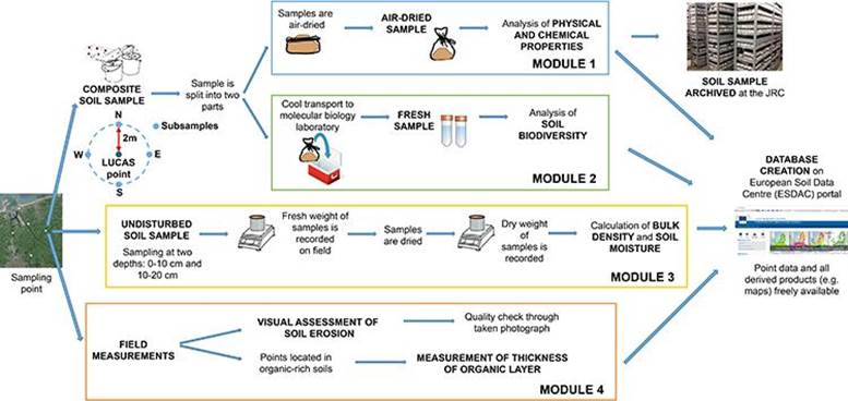
Fig. 5. LUCAS Soil workflow from sampling to database generation (A. Orgiazzi, et al., 2018).

The attempt to evaluate the SOC in European soil using the LUCAS database and NIR spectroscopy was published by Antoine Stevens, et al., 2013. In this study the accuracy to predict SOC content of different algorithms was tested to evaluate the potential of using the LUCAS soil database and to cover soil heterogeneity. Several performance parameters were analyzed and the best spectroscopic models having the highest parameter scores were chosen. These were then tested again by using a separate test set. It was observed that the accuracy of the predictions of SOC highly depended on soil classes (cropland, grassland, woodland mineral, and organic) and the use of auxiliary predictors (sand and clay). The results of the tests \96 performance parameter values, are shown in Table 3.

Table 3. Performance of the best spectroscopic models as measured against the test set (Antoine Stevens, et al., 2013).

Subset	Treatment^a	MVC^b	Predictor^c	SD^d	RMSEP^e	Bias^f	SEP-b^g	RPD^h	R^2	N^i
Cropland	SG1	svm	spc	8.6	4.9	0.2	4.9	1.74	0.67	2828
Cropland	SG1+SNV	svm	rfe+clay	8.6	4.0	0.1	4.0	2.17	0.79	2828
Grassland	SG1	svm	spc	17.4	9.3	-0.9	9.3	1.86	0.71	1383
Grassland	SG0	cubist	rfe+sand	17.4	6.4	0.1	6.4	2.7	0.87	1383
Woodland	SG1	svm	spc	29.8	15.0	0.8	15.0	1.99	0.75	1564
Woodland	SG0	cubist	rfe+sand	29.8	10.3	1.1	10.3	2.88	0.89	1564
Mineral	SG1	svm	spc	19.1	8.9	0.2	8.9	2.13	0.78	6053
Mineral	SG1	svm	rfe+sand	19.1	7.3	0.1	7.3	2.62	0.86	6053
Organic	SG1+SNV	cubist	spc	100.8	50.6	-10.9	49.5	1.99	0.76	368

^aSpectral transformation (SG0 = Savitzky-Golay smoothing; SG1 = Savitzky-Golay first derivative; SNV = standard normal variate);

^bMultivariate Calibration Model (svm = support vector machine regression; cubist = Cubist);

^cPredictor used in the models (spc = spectral matrix; rfe = spectral matrix with bands selected by recursive feature elimination);

^dStandard Deviation of the observations (g\B7kg^-1);

^eRoot Mean Square Error of Prediction (g\B7kg^-1);

^fBias (g\B7kg^-1);

^gStandard Error of Prediction (g\B7kg^-1);

^hRatio of Performance to Deviation;

ⁱNumber of validation samples.

As the authors of the study state all the models have shown limited accuracy in predicting the values of SOC. This suggests that accurate SOC predictions based on large scale spectral libraries can be hard to achieve. Prediction errors were found to be related to SOC variation, SOC distribution (skewness) and variation in other soil properties such as sand and clay content. The authors state that VIS-NIR spectral data alone may not be able to contain enough information to get accurate predictions of soil properties at large scales. Therefore, other strategies that can address this issue, such as the use of additional predictors in the modeling should be taken. However, other studies have gotten better results. For example, algorithm of partial least squares regression (PLSR) was applied together with the LUCAS database and remote Airborne Prism Experiment (APEX) spectral data in order to create a model for SOC estimation in the croplands of Luxembourg and Belgium (Fabio Castaldi, et al., 2018). In this study a so-called bottom-up analysis approach was taken. According to the authors, such an approach avoids the main errors which arise because large spectral libraries are built collating local libraries that were collected under differing conditions and using different protocols and instruments. This approach predicts the SOC values at sampling points based on the LUCAS spectral library. Then these values were linked to the airborne spectra building a PLSR model. Finally, the PLSR model was applied to all bare soil pixels of the airborne image producing SOC maps with the same spatial resolution as the airborne data. Thus, this approach allows laboratory analysis of the target variable to be avoided. The accuracy of the proposed method was compared with the traditional approach - the calibration of a multivariate model which links remote spectra and the quantity of the SOC measured in the laboratory. The flowchart of the proposed analysis method is presented in Fig. 6.

Fig. 6. The bottom-up approach proposed by Fabio Castaldi et al., 2018.

The main difference between the traditional and bottom-up approaches is that the latter does not require analytical laboratory measurements. Instead, different soil variables are estimated exploiting laboratory spectral data. The bottom-up approach consists of two main steps:

1. The estimation of a soil variable at sampling points exploiting the LUCAS spectral library and its ancillary data.
2. The mapping of the soil variables using remote-sensing data.

Artificial neural networks were employed for the creation of the mathematical models for SOC evaluation. NDVI was calculated in order to distinguish between the hyperspectral imaging pixels representing vegetation and soil. The results of this research have shown that the proposed bottom-up approach can provide the results of SOC analysis in comparison to the standard approach involving the testing of the soil samples in the laboratory and correlating the results with the data from the remote hyperspectral imaging.

A rather complex and large study was performed in order to analyze the differences in the spectral data provided by hyperspectral and multispectral imaging satellites and to estimate the best approach for SOC evaluation (D. \8Ei\9Eala, et al., 2019). The study was conducted in the Chernozem region of Czechia. Field sampling and predictive modeling of the spectral data was performed. The spectral data was collected from multispectral Sentinel-2, Landsat-8, and PlanetScope satellites, and multispectral Parrot Sequoia UAV. Aerial hyperspectral CASI 1500 and SASI 600 data was used as a reference. The data processing steps were as follows:

1. Pixels in individual data sources were filtered based on NDVI value. The threshold was set to 0.25.
2. The filtered dataset was partitioned into a training set and a test set.
3. A mathematical model was trained using the training set. Several models were tested and the final model was selected based on the smallest value of root mean square error of cross-validation.
4. The accuracy of prediction was evaluated by determining the measure of accuracy computed based on a comparison of observed and predicted values of the validation set.
5. Finally, the best model was applied to the entire dataset of image spectral data.

The results of the study have shown that very similar prediction accuracy for all spaceborne sensors with only minor prediction variance can be obtained. The results of the SOC mapping with the data from different imaging systems are presented in Fig. 7.\A0\A0\A0\A0\A0\A0\A0\A0

Fig. 7. SOC maps calculated using different remote sensing platforms (D. \8Ei\9Eala, et al., 2019).

Several other studies have tested the efficiency of the mathematical algorithms for soil analysis and organic carbon concentration evaluation. A study done in Greece (P. Tziachris, et al., 2019), have compared several machine learning algorithms and found that the result of the SOC evaluation is dependent on the algorithm choice. It was determined that algorithms such as Random Forest or Gradient Boosting show better accuracy than other methods like Ordinary Kriging. A review on the different algorithms used for determination of SOC content (S. Lamichhane, et al., 2019) has also evaluated that machine learning algorithms provide more accurate results. This study has also looked into the environmental covariates which are most important for one of the machine learning algorithms (Random Forest). Covariates representing organism activities were the most frequent among the covariates, followed by the variables representing climate and topography. Climate was reported to be influential in determining the variation in SOC level at regional scales, followed by parent materials, topography and land use. However, for mapping at a resolution that represents smaller areas such as a farm- or plot-scale, land use and vegetation indices were stated to be more influential in predicting SOC. Similar conclusions were drawn in another study written by T. Angelopoulou, et al., 2020. The authors find that the results of spectral SOC estimations are promising but more research needs to be done in terms of selecting the spectral range, preprocessing methods, and the calibration techniques. Also, as already mentioned a specific importance should be kept on covariates such as soil moisture, soil roughness, vegetation cover, and others that affect SOC spectral response. Authors stated that various inconsistencies among studies should be solved. Therefore, when publishing results more information should be included about the experimental design, the criteria used for the selection of the chemometric approach, and the pre- and post- processing procedures in order to facilitate comparisons of results among studies.

A lot of effort is being put in order to create the best tool for SOM evaluation from the spectroscopic data. However, there is no census on what approach is the best as we can see from the various publications and performed studies. Still a lot can be learned to take the best approach possible at this time. What has to be taken into account first is that spectral regions which can be used to quantify soil organic carbon (SOC) are located mainly in broader bands in the visible region of the spectrum and in the narrower bands of the SWIR spectrum (between 1600 and 1900 nm and around 2100 and 2300 nm). Because of that, the spectral resolution of the sensors significantly influences the quality of SOC predictions. Because of that it is necessary to use data with appropriate spectral resolution taken across the VNIR-SWIR spectrum for accurate SOC estimates. Second, a well thought out method for processing the data should be used. Usually, different thresholds of vegetation indices are used for identifying and removing unwanted pixels in the image. Mainly NDVI for green vegetation, NBR2, or MID-infrared for non-photosynthetic vegetation or combined indexes, such as Bare soil index (BSI) or PV are used. Also, statistical parameters \97 mean, median, or minimum or other methods used that improve the image values are used. These for example, can be application of PCA components, calculation of standard deviation or using low-pass filter. Furthermore, it is necessary to develop new algorithms, not only for identifying bare soils, but also for removing the influence of moisture, surface roughness, or vegetation residues. Clouds and unwanted shades also affect the input data and should also be taken into account. Lastly, the lack of comparability between different studies is a big issue. Model evaluation and accuracy is investigated using different methods. Thus, different studies are deprived of certain information which is essential for the comparison between the results. What is more, different laboratories used different protocols for soil sampling and measurements together with different instrumentation. These factor in and hinder the reliability of the results. To tackle this challenge a unified soil spectral library (SSL) potentially could be a strong boost towards a more accurate prediction of SOM.